How to use the functions of data handling using VLOOKUP Excel function

If the amount of data is huge, and you have to find any information, the usual search is not convenient to use. And here you find VLOOKUP (in order to find data in a column) or HLOOKUP (in a row). To use these functions it's possible only on the case when the information is not repeated.

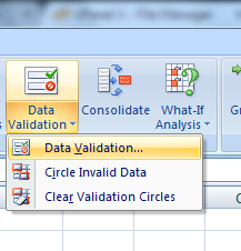
First of all, it's necessary to create a field with a list. Here its' better to use a blank sheet, in order to display all the target information in it. Choose the following menu options: Data – Data validation – Data validation...

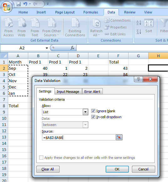
In the open window select Settings – Allow – List. The filed Source will appear, where it's necessary to point the link for the range of the cells.

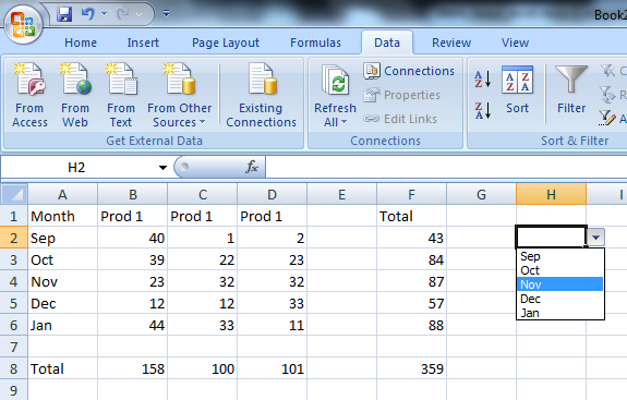
As a result, we get the dropdown list.

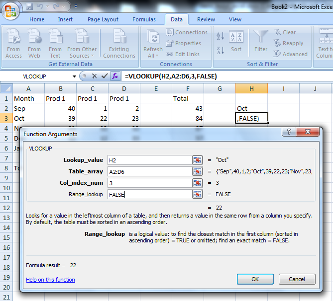
The next step is making a function. You should make the cell active, where you want the result of our search to be displayed. Then press the option of the formula – Insert function – VLOOKUP. Here you have to input the following values.

• Lookup_value – refer to the cell where we have just placed the dropdown list.
• Table_array – this is our table with the data, and it should be selected so that the search argument (according to which we created the dropdown list) should be located in the first column. Now we have to make the reference absolute. For this purpose we use the key F4 or input the signs $. Selection of the table is made without the heading, but just the data.
• Col_index_num – the number should be specified as per the column order, including the data that we want to see in the result of our search.
• Range_lookup – FALSE, because we need the exact matching of the data with that one that is set in the search.

It's possible to change the number of the column in the function VLOOKUP and to make a selection in different columns.