Excel Techniques for Sorting Teams in a Group Round (Part 1)

We get asked quite frequently for a password to unblock the sports calendar in order to study through the formulas. As a rule, the formulas in the calendar are uneasy and sometimes complicated. Hence, in this article we will discuss the major techniques used for sorting the football teams in a group tournament.

Let's start from creating a new Excel file and prepare the data for tournament results. Let's say we have 2 groups with 4 teams per each (Group-A teams: Alpha, Beta, Gamma, Delta and Group-B: Epsilon, Zeta, Eta, Theta), where each team is supposed to play one match with all three competing teams.

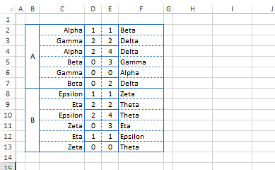
Let's prepare the tables, where it is possible to see the results of sorting teams according to the matches played:

First of all, for each match it is required to define the result: Win/Lose/Draw. It is not difficult to verify with help of "IF" function:

=IF(D2>E2, "WIN", IF(D2<E2, "LOSE", "DRAW"))

The formula checks, whether the first team has scored more goals and then the result is "WIN" if the second team scored more, then the result is "LOSE" and "DRAW" in case if the amount of goals is the same. However, for future calculations we are required to know the team name, so that it becomes possible to create a line, such as below:

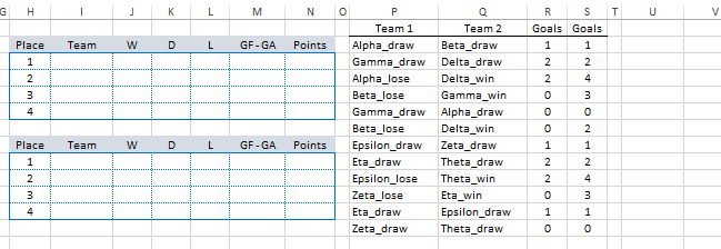
TEAM_NAME_win, TEAM_NAME_lose, TEAM_NAME_draw

=C2 & IF(D2>E2,"_win",IF(D2<E2,"_lose","_draw"))

This functions has got only one flaw: it will work for empty cells as well, i.e. the result will be displayed as "TEAM_NAME_draw" until the outcome of the match is unknown. Hence, let's add a verification to ensure that both values of match goals were keyed-in:

=C2 & IF(OR(D2="",E2=""),"",IF(D2>E2,"_win",IF(D2<E2,"_lose","_draw")))

Now if the match result is not keyed-in or only one team's goals are entered, then the cell will simply have the "TEAM_NAME" value. By analogy, let's construct the function for the second team participating in the match, while not forgetting to change the comparison signs:

=F2 & IF(OR(D2="",E2=""),"",IF(D2<E2,"_win",IF(D2>E2,"_lose","_draw")))

In order to calculate the goal difference and conceded goals we will also need the results. However, let's duplicate these values in separate columns in order to verify the accuracy of keyed-in data with help of formulas below:

=IF(OR(D2="",E2=""),0,D2)
=IF(OR(D2="",E2=""),0,E2)

The data of this formulas are to be copied for all 12 matches, followed by sorting.

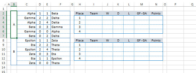
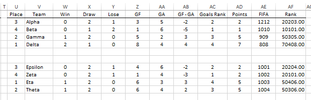
The calculation of intermediate data (number of victories, draws, losses and goal difference) is to be done in a separate table (U:AG). The results of that table are to be displayed in a sorted form in columns H:N.

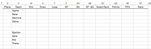
The calculation of victories amount is to be done with help of COUNTIF formula, e.g. the formula for Alpha team is as follows:

=COUNTIF(P:Q,"Alpha_win")

i.e. we calculate how many times the Alpha_win line appears in the column of matches results (P:Q). However, in order not to key-in such formulas for each team separately, let's create a line "Alpha_win" for each team with help of the formula below:

=COUNTIF(P:Q,V2 & "_win")

Analogically, let's carry out the calculation of draws and losses amount. The next stage is the calculation of scored/conceded goals for each team. SUMIF formula is used as follows:

=SUMIF(C:C,V2,R:R) + SUMIF(F:F,V2,S:S)

Conceded goals are calculated in similar manner – we just change the columns to be summed.

At this stage we can calculate the amount of scored points for each team (3 points for a win, 1 for a draw) as well as the goal difference. Likewise, we have reached the moment when it is required to bring it all to a common factor and define the position within a group where the team is. It is one of the key moments and the "RANK" function will be very useful in this case. However, it is required to assign each team with some index, according to which the ranking is to be done. The idea of such index is included in constructing of a formula as follows:

POINTS * 10000 + GOAL_DIFFERENCE * 100 + GOALS_F

i.e. the team with higher amount of scores will have a higher index, while in case if the scores are equal, then the index will be influenced by other results, such as goal difference, total amount of scored goals etc. Since the goal difference can have a negative value, then we will use the value of "RANK" function for such indexes instead of the difference itself in order to avoid the errors. In addition, until no results are keyed-in, this index will be equal to zero for all teams and "RANK" function will have the same output equal to 1 for all teams, while we need to receive all 4 values (1, 2, 3, 4) in order to avoid ambiguity in sorting. Hence, let’s use the FIFA index for each team (it is always different) and divide it by quite a big number, so that it has the smallest influence on the index. As result, we will get the estimated index for each team as follows:

POINTS * 10000 + GOAL_DIFF_RANK * 100 + GOALS_F + FIFA/1000000

Or in a form of a formula in the column AF:

=AD2*10000 + AC2*100 + Z2 + AE2/1000000

Now we can define the position of each team within a group by using the RANK function (in the column U):

=RANK(AF2,AF2:AF5,0)

The last parameter here is responsible for the type of sorting. We use 0 for the declining sorting, i.e. the team with the highest index in the column AF will have the value equal to 1 (first place)

The final part includes the output of the sorted result in the report table (columns H:N). VLOOKUP function is used for that (value, table, column, FALSE). It searches the line in the first column with desired value value in a given table table and returns the value from the column column. Likewise, the first team in the table will have the following formula:

=VLOOKUP(1,U2:AF5,2,FALSE)

By analogy, let's create a formula to output the number of wins, draws, goal difference and total score (only the value of the column to be returned (column) will vary in the formula). Only the desired value (value) will vary in the formula for the 2nd, 3rd and 4th place of a team.

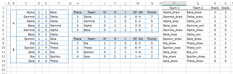
By now it should be clear that the calculated place in a group was placed in the very beginning of the intermediate table (in the column U) exactly for use of VLOOKUP formula. "RANK" function was introduced only in Excel 2007 and above, hereby in earlier versions there was used a trick with help of a "COUNTIF" function. For example, you can check the formula in the column AG:

=5 - COUNTIF(AF2:AF5,"<="&AF2)

The sorting is complete, but, of course, it has got a flaw – in case if the indexes are equal (points and goal difference), then the teams are sorted according to FIFA rating, which is wrong, because their individual matches should be considered first of all. We will discuss the ways to resolve that in our next article.

Download: Sorting Teams in a Group Round - Excel File (15Kb)