Advanced Filter Excel Template
Quite often Excel is used for working with small databases and spreadsheets with up to several tens (or hundreds) of thousands of rows. Such tools as Pivot Tables, filters and Advanced Filters are used for easy and convenient data analysis.
Advanced Filter allows a data sampling function to be performed from Excel spreadsheets which is similar to SQL-query. Typically, there are two additional rows: the top row that contains a field name (a heading) and the bottom value based on which the data will be filtered. All values can be defined either as a target value or specified in the comparison form: "more" (>100), "less" (<200), or text values, that contain a part of the "*some text*".
For example, we are going to have a look at the spreadsheet with three thousands of rows (sheet "Data") and create the user-friendly form of data filtering (sheet "Filter").
The spreadsheet contains columns with the following data:
- Date
- Year
- Month
- Country
- Category
- Product
- Count
- Price
- Total
Data sampling will be organized according to the following data:
- Year
- Month
- Country
- Category
- Product
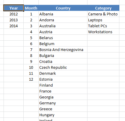
The list of available fields
First of all, we create the lists of permissible values for all fields, except "Product". Data, that contain the following words (*some word*), will be searched based on the "Product" field.
Data for the "Month" field is naturally defined – from 1 to 12. For the rest of fields, we will use the Advanced Filter function for filtering unique values. It can be done by calling out the dialog window in the Excel menu: Data->Sort &; Filter->Advanced:
- Select the "Country" column;
- Switch a radio-button to "Copy to another location";
- The "Criteria range" field should be empty;
- Select a cell, where data will be copied to "Copy to";
- And select "Unique records only".
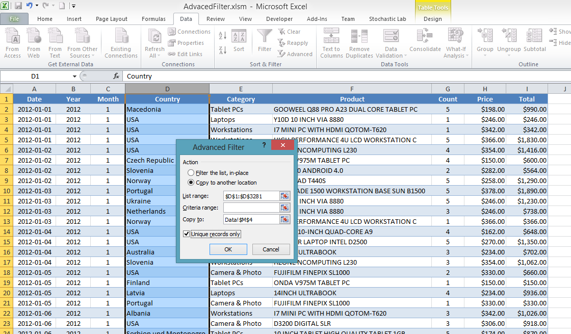
As a result, we get a list of all values in the field "Country" which we will be sorted alphabetically for more convenience.
Apply the same procedure to the fields "Year" and "Category".
Parameters for data filtering
The picture below shows an example of how cells with headings should be specified for the criteria of data filtering:
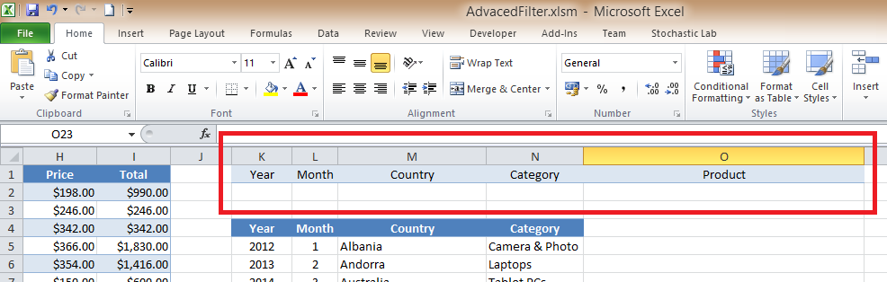
We will use the value of ">0" for the criteria "Year" and "Month", if the concrete field value is not specified:
=IF(Filter!D3="",">0",Filter!D3)
for the criteria "Country" and "Category" use "*":
=IF(Filter!D5="","*",Filter!D5)
for the "Product" field, a target value will be set between symbols "*":
=IF(Filter!D7="","","*"&Filter!D7&"*")
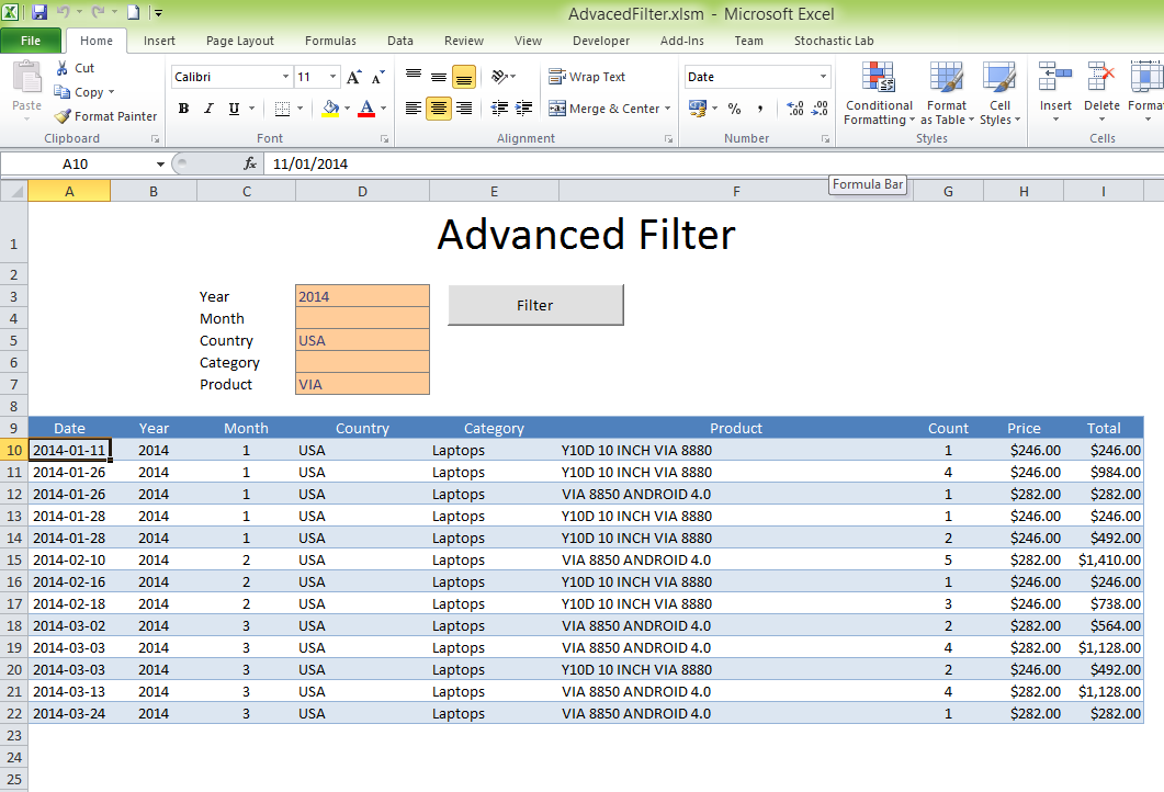
Form used for data sampling
Let's create a new "Filter" list with request parameters and prepared data sampling results as it is shown below:
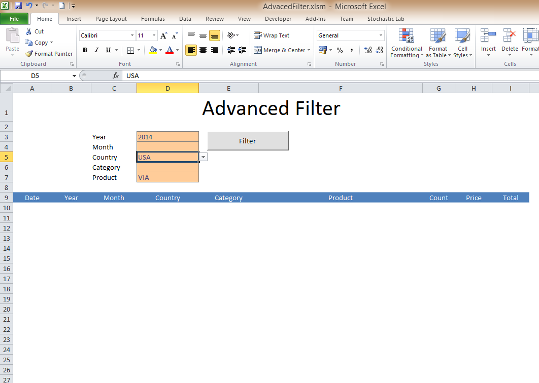
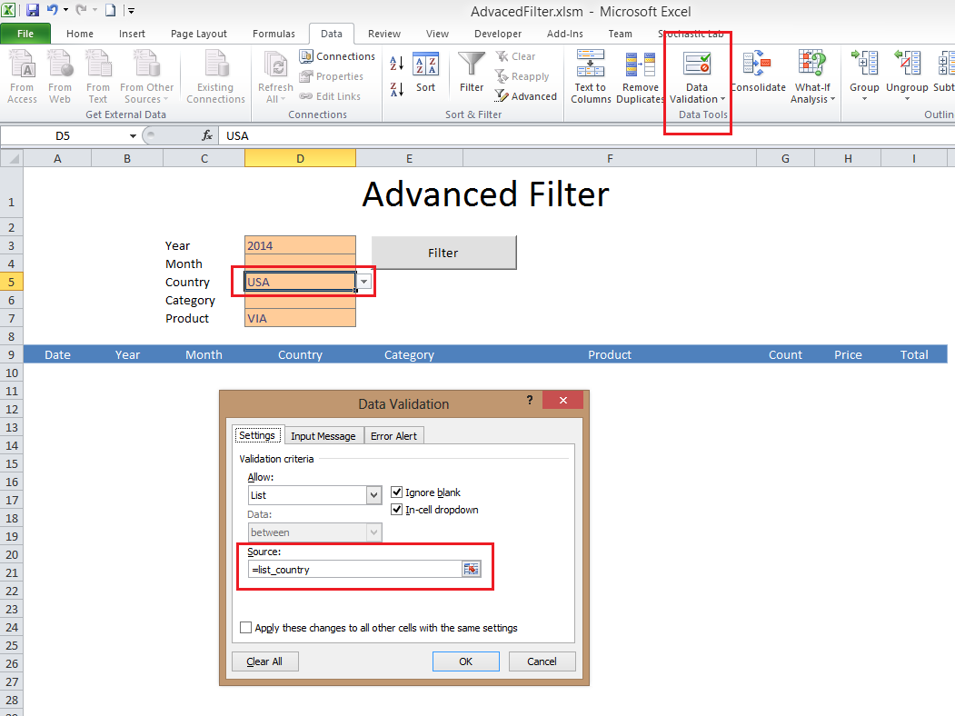
For the first four parameters we will limit the list of entered parameters by means of the "Data Validation" function. Moreover, it will allow you to use a drop-down list for the entered data:
- Define names for the following lists (sheet "Data"):
- Range K5:K7 – define a name: list_year
- Range L5:K16 – define a name: list_mth
- Range M5:K47 – define a name: list_country
- Range N5:K8 – define a name: list_category
- For each cell of request parameters we will define the most relevant list in the "Data Validation" dialog window.
Button for data filtering
Create a button "Filter" and write down a macro command for the data filtering according to the set criteria.
For example, the macro command will look like this:
Delete 9 rows given below:
' clear old data first
Dim n As Long
n = Cells(Rows.Count, "A").End(xlUp).Row
If n > 9 Then
  Rows("10:" & CStr(n)).Delete Shift:=xlUp
End If
Apply the filter with the following criteria:
With Sheets("Data")
  .Select

  ' apply filter
  .Range("A:I").AdvancedFilter Action:=xlFilterInPlace, CriteriaRange:=.Range("Criteria"), Unique:=False
End With
As a result of using the VBA-script, we will get a list of rows in the "Data" field that will fully satisfy our requirements. Now we will need to copy the data to the "Filter" list:
 ' select filtered rows
  Dim rngFilter As Range
  Set rngFilter = .Range("A2", .Cells(.Rows.Count, "A").End(xlUp)).Resize(, 9)

  ' copy selection
  rngFilter.Select
  Selection.Copy
End With

' paste new data
Sheets("Filter").Select
Sheets("Filter").Range("A10").Select
ActiveSheet.Paste
Application.CutCopyMode = False
Remove the filter and get the spreadsheet style back for more convenience:
' remove filter
Sheets("Data").ShowAllData

' table style
Sheets("Data").ListObjects("Table1").TableStyle = "TableStyleMedium2"
Attention! If there are no data given for some of the criteria values, the macro will automatically copy the whole spreadsheet. In order to avoid it, we should check the number of filtered rows. In this case, we will not copy the data if there are no rows available for data sampling.
  ' count number of filtered rows
  On Error Resume Next
  n = 0
  n = rngFilter.SpecialCells(xlCellTypeVisible).Rows.Count
  On Error GoTo 0

  If n = 0 Then
    Sheets("Filter").Select

    ' skip copying
    GoTo skip_copying
  End If
The full VBA script can be download and examined at the Advanced Filter Excel Template (220 Kb)